
EMG Filters
Every trace in every window may have up to six filter effects applied. The original data is subjected to the first enabled filter. The output from this filter is subjected to the next enabled filter and so on up to a maximum of six filters. The output from the final filter is displayed.
Each of the filters has the following options:
This filter simply converts a negative value to a positive value of the same magnitude. No filter constant is required.
A moving average filter may be applied to any waveform.
- When enabled, each point calculated in a trace is the average of a number of values up to and including the current point.
- The number of values is the filter constant and may be set from 2 samples upwards.
- The filter constant may be specified in samples or milliseconds where the number of milliseconds is the number of samples multiplied by (1000/sampling rate).
- The moving average generates as many outputs as inputs. For example, assuming a filter constant of 3, the following calculations are performed:
- Output 1 = Input 1
- Output 2 = Average of inputs 1 and 2
- Output 3 = Average of inputs 1, 2 and 3
- Output 4 = Average of inputs 2, 3 and 4
- Output 5 = Average of inputs 3, 4 and 5
- Output n = Average of inputs n-2, n-1 and n
HINT: The average filter is useful for reducing high frequency noise in a waveform. For example, if a heart beat trace that is sampled at 1000Hz contains 50Hz mains interference, it may be reduced by averaging over one mains cycle (1/50th second). One mains cycle corresponds to 20 samples (1000Hz sample-rate divided by 50Hz interference) so averaging 20 values will reduce the noise significantly. Note that averaging over 40, 60, 80, … samples will also reduce the noise but it may also reduce the signal of interest.
Each sample of data is first squared and then a moving average is taken of these squares. The output is the square root of each average calculated.
- The filter constant may be specified in samples or milliseconds where the number of milliseconds is the number of samples multiplied by (1000/sampling rate).
The velocity filter involves calculating the rate of change of data at every data point. This is effectively the gradient of the tangent to the line at that point.
To obtain a suitable gradient, a least-squares method is used to estimate a straight line using the data either side of the data point being calculated. The gradient of this line is the filter output.
- The filter constant defines the number of data points used in the least squares line estimation. It may be specified in samples or milliseconds where the number of milliseconds is the number of samples multiplied by (1000/sampling rate).
- Using this filter will alter the displayed units. For example, if the original units are degrees then the filtered units will be degrees/sec.
The integrate filter calculates the area under the graph from the start up to the point being displayed. This filter often produces a rapidly rising/falling graph when the data is not centerd on zero.
- The filter constant defines a divider used to reduce the calculated area for each point. This is useful when the data would otherwise produce an integrate output that is too large to display.
- Using this filter will alter the displayed units. For example, if the original units are degrees then the filtered units will be degrees-sec.
The offset filter simply adds or subtracts a percentage of full scale from every data point. This may be used to alter or redefine the null or zero point for each trace. This has the effect of moving the trace up or down in the window.
- The filter constant defines percentage of full scale and may be positive or negative.
The scale filter simply multiplies every data point by a percentage of full scale. This has the effect of increasing or decreasing the size of a trace in the window.
- The filter constant defines percentage of the original value. Constants less than 100% will reduce the amplitude of the trace whilst constants more than 100% will increase the amplitude of the trace.
The median frequency is calculated for a block of samples whose length is defined by the filter constant. This calculation is repeated as necessary across the trace and the resulting frequencies plotted as a series of lines connecting the calculated median frequencies. The following steps are performed:
- A block of samples defined by the filter constant is taken and zero padded to the nearest power of 2.
- A Windowing function applied to the data as specified by the selection at the bottom left of the Settings Window. See Using FFT Windowing Functions for more information.
- An FFT is performed and, if selected, FFT High Pass Filters are used to Remove DC and to Remove Very Low Frequencies from the calculations. Note that a large DC component can seriously degrade the accuracy of the median frequency calculation.
- The amplitude magnitude of each FFT output frequency is squared.
- The median frequency is determined such that the area of the amplitude-squared frequency graph below the median frequency is the same as above the median frequency i.e. there is equal power either side of the median frequency.
- The process is repeated for the next block of samples.
The mean frequency is calculated for a block of samples whose length is defined by the filter constant. This calculation is repeated as necessary across the trace and the resulting frequencies plotted as a series of lines connecting the calculated mean frequencies. The following steps are performed:
- A block of samples defined by the filter constant is taken and zero padded to the nearest power of 2.
- A Windowing function applied to the data as specified by the selection at the bottom left of the Settings Window. See Using FFT Windowing Functions for more information.
- An FFT is performed and, if selected, FFT High Pass Filters are used to Remove DC and to Remove Very Low Frequencies from the calculations. Note that a large DC component can seriously degrade the accuracy of the mean frequency calculation.
- An FFT is performed and all frequencies below (maximum frequency / 50)Hz are rejected; this corresponds to 10Hz at 1000 samples / second.
- The amplitude magnitude of each FFT output frequency is squared.
- The mean frequency of the resultant amplitude-squared against frequency graph is determined.
- The process is repeated for the next block of samples.
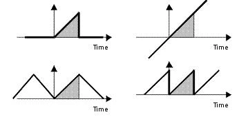
When data is captured, a 'window' is effectively opened on the signal to view the waveform for a period before the 'window' is closed again. Before and after the window is open, the FFT calculation has no idea about the value of the signal. For example, the four waveforms shown right contain the same captured data (shown in grey) but have different frequency contents.
An FFT assumes that the data sequence is part of a signal that repeats periodically as illustrated by the sawtooth waveform on the lower right of the above diagram. The consequence of assuming a periodic continuation of the underlying signal is that if the amplitude at the start and the end of the sample of data are not equal then the signal will be analyzed to contain a discontinuity, whether the signal has such a discontinuity or not. Since sharp discontinuities have broad frequency spectra, these will cause the signal's frequency spectrum to be spread out. The spreading means that signal energy that should be concentrated only at one frequency, instead, leaks into all the other frequencies. This spreading of energy is called 'spectral leakage'. Since spectral leakage is related to discontinuities at the ends of the measurement time, it will be worse for signals that happen to fall such that there are large discontinuities
This is a problem since the FFT will only be an accurate calculation of the frequency content if the captured data is one or more complete cycles of a periodic underlying signal. This is normally not the case.
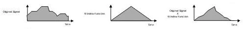
In order to improve the accuracy of the FFT, it is normal practice to multiply the sampled data by a window function before implementing the FFT. This window function is a series of numbers that are usually symmetrical with the mid-point of the sample time range and have a mid-point value of one e.g. the Triangle or Bartlett window.
A number of window functions are possible including a Rectangular Window that does not actually change the data at all. Some of the window functions provided are:
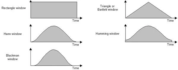
In order to compare the different windows, they may be plotted on the same axis as follows:
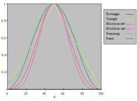
The choice of window function is usually made after some experience processing the type of signals being used. However, some guidelines can be given:
- Use a rectangular window for transient signals;
- Hann (von Hann) and Hamming for continuous waveform data;
- Rectangular (Flattop) for accurate amplitude measurements or
- Blackman for maximum frequency resolution.